IB DP Environmental Systems & Societies
Individuals, Populations,
Communities & Ecosystems
Subtopic 2.1 — New Syllabus (First Assessment 2026)
Standard Level + Higher Level
2.1.1
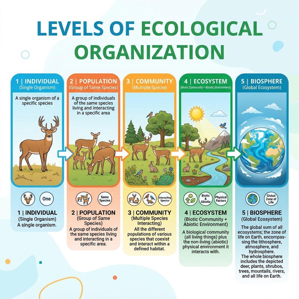
Levels of Ecological Organization
2.1.2
Individual Organisms
What Makes an Individual?
- A single, discrete living thing — one plant, one animal, one bacterium
- Belongs to a particular species — a group of organisms that can interbreed and produce fertile offspring
- Has unique characteristics (phenotype) influenced by its genetics (genotype) and environment
- Interacts with its environment — responds to abiotic and biotic stimuli
Example: A single oak tree (Quercus robur) is an individual belonging to the species Quercus robur.
2.1.3
Classification of Organisms
Mnemonic: "King Philip Came Over For Good Spaghetti"
Why Classify?
- Organizes vast biodiversity into manageable groups
- Predicts characteristics of new species based on relatives
- Enables communication between scientists worldwide
- Reveals evolutionary relationships
Binomial Nomenclature
Every species gets a two-part Latin name: Genus + species
e.g., Homo sapiens, Panthera leo, Rosa canina
Genus is capitalized; species is lowercase. Both are italicized.
2.1.4
Tools for Identification
| Tool/Method | What It Does | Example |
|---|---|---|
| Dichotomous keys | Step-by-step decision tree based on observable traits | Leaf shape → flower colour → bark texture |
| Morphological analysis | Comparing physical structures | Skeleton comparison, wing venation |
| Microscopy | Examining cellular/microscopic features | Pollen grain structure, diatom shells |
| DNA barcoding | Comparing short genetic sequences to reference databases | COI gene for animals, rbcL for plants |
| Chemical analysis | Identifying unique biochemical markers | Protein electrophoresis, chromatography |
| Ecological niche | Role and habitat help narrow identification | Nocturnal raptor in tropical forest |
2.1.5
What Is a Population?
The Four Criteria
- Same species
- Same area (geographic location)
- Same time
- Capable of interbreeding
Examples
- All blue whales in the Pacific Ocean
- All dandelions in a school field
- All bacteria of species E. coli in your gut right now
2.1.6
Distribution: Abiotic & Biotic Factors
Abiotic Factors
- Temperature — affects enzyme activity and metabolism
- Sunlight — energy for photosynthesis; drives behaviour
- pH — affects soil chemistry and aquatic life
- Salinity — freshwater vs marine species tolerance
- Dissolved oxygen — essential for aquatic organisms
- Soil texture — determines water retention, root growth
- Water availability — precipitation, humidity
Biotic Factors
- Food availability — predator/prey abundance
- Competition — for resources, territory, mates
- Predation — presence of predators
- Disease/parasites — population health
- Mutualism — beneficial relationships
- Human activity — habitat modification
2.1.7
Abiotic Factors in Detail
How Abiotic Factors Set Limits
Every species has a tolerance range for each abiotic factor — the range within which it can survive, grow, and reproduce. Outside this range, the species cannot persist.
Temperature
Tropical corals: 23–29°C only. Beyond this → bleaching and death.
Salinity
Freshwater fish (0–0.5 ppt) vs marine fish (30–40 ppt). Stenohaline species tolerate narrow ranges.
Dissolved O₂
Cold water holds more O₂. Trout need >6 mg/L; carp tolerate >2 mg/L.
2.1.8
The Ecological Niche
What a Niche Includes
- Habitat: where the organism lives
- Diet: what it eats and what eats it
- Activity patterns: when it is active (diurnal/nocturnal)
- Reproduction: breeding season, mate selection
- Abiotic requirements: temperature, moisture, pH range
Habitat vs Niche
Habitat = the "address" — where an organism lives
Niche = the "job description" — the full role it plays in the ecosystem
Two species can share the same habitat but have different niches (e.g., a robin and a hawk both live in a forest, but eat different things).
2.1.9
Population Interactions
| Interaction | Type | Effect on A | Effect on B | Example |
|---|---|---|---|---|
| Predation | +/− | Predator gains energy | Prey killed | Lion → zebra |
| Herbivory | +/− | Herbivore gains energy | Plant tissue lost | Caterpillar → leaf |
| Parasitism | +/− | Parasite gains nutrients | Host harmed | Tick → deer |
| Mutualism | +/+ | Both benefit | Both benefit | Bee ↔ flower |
| Competition | −/− | Reduced resources | Reduced resources | Lions vs hyenas |
| Disease | +/− | Pathogen reproduces | Host weakened/killed | Malaria → human |
2.1.10
Carrying Capacity
What Limits Population Size?
- Food supply — limited energy available
- Water — especially in arid environments
- Shelter/nesting sites — physical space
- Predation pressure — more prey → more predators → population control
- Disease — spreads faster in dense populations
- Waste accumulation — toxic buildup in closed systems
2.1.11
Density-Dependent Regulation
Density-Dependent Factors
Effects that increase with population density:
- Competition intensifies as density rises
- Disease spreads faster in crowded populations
- Predation increases with prey density
- Waste/toxins accumulate faster
Negative Feedback
A stabilizing mechanism where the output counteracts the change:
↓ Population → ↓ Competition → ↓ Death rate → ↑ Population
2.1.12
Exponential vs Logistic Growth
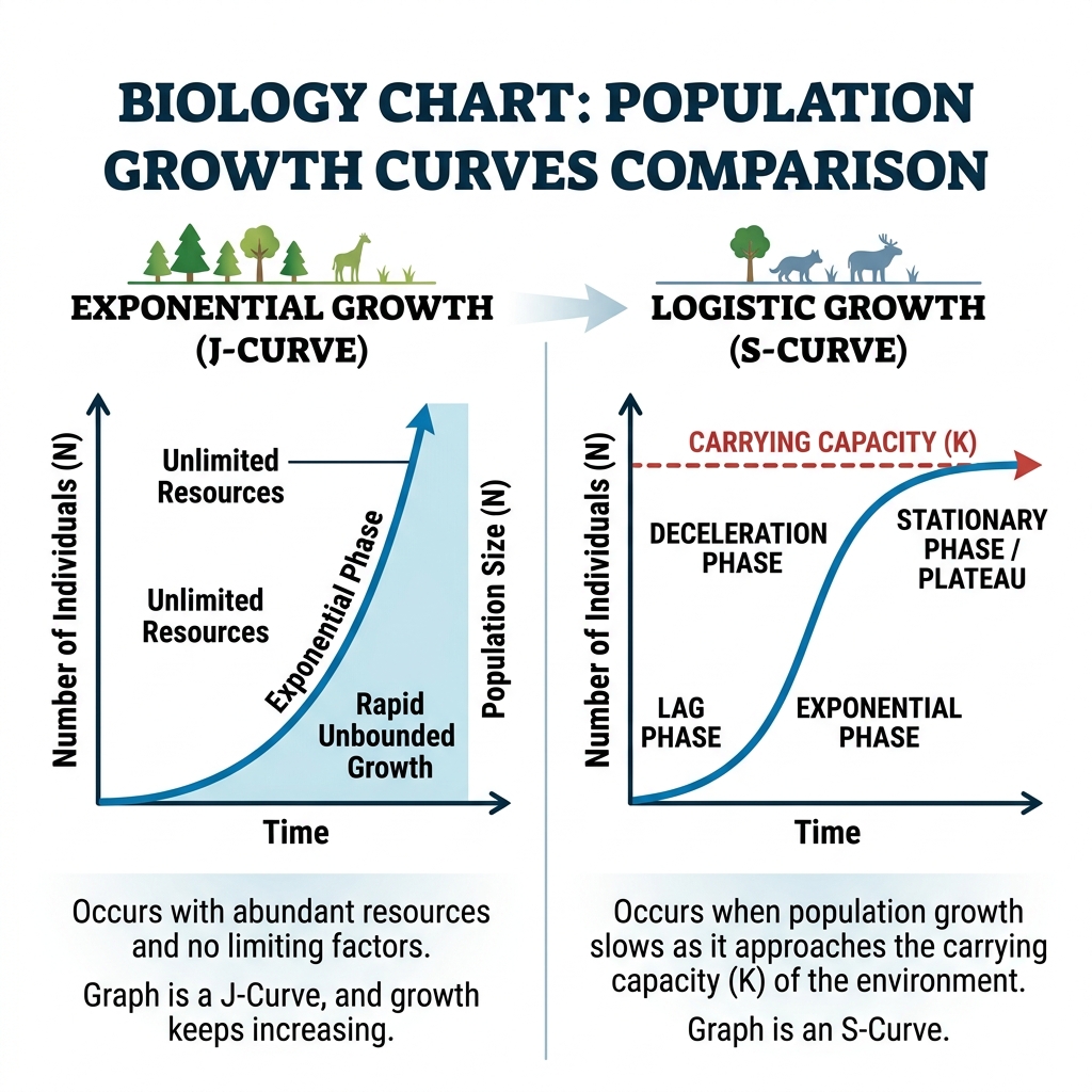
Exponential Growth (J-curve)
Unlimited resources → constant growth rate → population explodes
r = intrinsic rate of increase
Only occurs temporarily
Logistic Growth (S-curve)
Limited resources → growth slows as N → K → stabilizes
(1 − N/K) = the braking factor
Realistic model for most populations
2.1.13
Human Population Growth
| Limiting Factor | How Humans Overcame It | Consequence |
|---|---|---|
| Famine | Agriculture, food technology, global trade | Population explosion |
| Disease | Medicine, vaccines, sanitation | Increased life expectancy |
| Predation | Technology, weapons, habitat dominance | No natural predators |
| Natural disasters | Engineering, early warning systems | Reduced mortality |
2.1.14
Human Carrying Capacity
Why Is It So Hard to Calculate?
- Technology changes: Green revolution, fossil fuels, GMOs constantly shift what's "possible"
- Trade: Humans import resources globally, masking local overpopulation
- Inequality: 1 American uses as many resources as 30+ people in developing nations
- Time lag: Environmental degradation may not manifest for generations
- Complexity: Humans affect multiple ecosystems simultaneously
2.1.15
Sampling Population Abundance
Random Sampling
Quadrats placed at random coordinates. Each location has equal chance.
Use for: stationary organisms
Systematic Sampling
Quadrats at regular intervals (e.g., every 5m). Covers area evenly.
Use for: uniform habitats
Transect Sampling
Counted along a line or belt. Shows distribution changes along gradients.
Use for: zonation studies
2.1.16
Random Quadrat Sampling
Procedure
- Define the study area (e.g., a meadow of 100m × 100m)
- Generate random coordinates using a random number table or calculator
- Place a quadrat frame (e.g., 0.5m × 0.5m) at each random point
- Count all individuals of the target species within each quadrat
- Repeat for multiple quadrats (minimum 10 for reliability)
- Calculate the mean per quadrat and extrapolate to the whole area
2.1.17
Capture-Mark-Release-Recapture
Lincoln Index Method
- Capture a sample of individuals (first catch)
- Mark them (non-harmful tags, paint, clip)
- Release them back into the population
- Wait for them to mix with the population
- Recapture a second sample
- Count how many in the second sample are marked
Worked Example
First catch: 50 marked and released. Second catch: 40 total, of which 10 are marked.
N = (50 × 40) ÷ 10 = 200 estimated individuals
2.1.18
What Is a Community?
Community Properties
- Species composition: which species are present
- Species diversity: richness + evenness
- Trophic structure: who eats whom
- Interaction web: all biotic interactions
Community vs Ecosystem
Community = all living populations in an area
Ecosystem = community + all non-living components
2.1.19
Habitat
| Term | Definition | Analogy |
|---|---|---|
| Habitat | The physical place where an organism lives | The "address" |
| Niche | The role and requirements of an organism | The "job description" |
| Range | The geographic area where a species is found | The "neighbourhood" |
2.1.20
Ecosystems as Open Systems
Energy Flows Through
- Input: Solar radiation
- Through: Producers → Consumers → Decomposers
- Output: Heat (infrared radiation)
- Energy is not recycled
Matter Cycles Within
- Input: Atmospheric gases, precipitation
- Through: Biogeochemical cycles (C, N, P, H₂O)
- Output: Runoff, gas exchange
- Matter is recycled via decomposition
2.1.21
Sustainability as a Natural Property
- Negative feedback loops maintain equilibrium
- Nutrient cycling ensures matter is recycled
- Biodiversity provides resilience
- Succession allows recovery after disturbance
- Carrying capacity regulates population size naturally
2.1.22
Tipping Points in Ecosystems
Examples
- Coral reef bleaching: sustained warming → coral death → algae-dominated reef
- Lake eutrophication: nutrient overload → algal bloom → oxygen depletion → fish death
- Amazon dieback: deforestation + drought → forest → savanna
Why Tipping Points Matter
- Often irreversible on human timescales
- Difficult to predict precisely
- Can cascade through connected ecosystems
- Loss of ecosystem services affects humans
2.1.23
Keystone Species
Classic Example: Sea Otters
Sea otters prey on sea urchins. Without otters, urchin populations explode and destroy kelp forests.
🦦 Otters removed → urchins overpopulate → kelp forest destroyed → ecosystem collapses
Other Keystone Examples
- Wolves in Yellowstone: controlled elk → vegetation recovered
- Elephants in savanna: maintain grassland by felling trees
- Beavers: create wetland habitats for countless species
Conservation Implication
Protecting keystone species can be more effective than protecting many less impactful species. Removing a keystone can trigger cascading extinctions.
2.1.24
Planetary Boundaries
| Boundary | Status |
|---|---|
| Biosphere integrity (genetic diversity) | ⚠️ CROSSED |
| Biosphere integrity (functional diversity) | ⚠️ CROSSED |
| Biosphere integrity (land-system change) | ⚠️ CROSSED |
| Biosphere integrity (freshwater change) | ⚠️ CROSSED |
| Biosphere integrity (biogeochemical flows – N) | ⚠️ CROSSED |
| Biosphere integrity (biogeochemical flows – P) | ⚠️ CROSSED |
| Climate change | ⚠️ CROSSED |
| Novel entities (chemical pollution) | ⚠️ CROSSED |
| Stratospheric ozone depletion | ✅ Within safe space |
2.1.25
Reversing Biosphere Integrity Loss
- Halt biodiversity loss: protect endangered species and habitats
- Restore degraded ecosystems: reforestation, wetland restoration, coral rehabilitation
- Reduce pollution: limit chemical and plastic inputs
- Sustainable land use: reduce deforestation, promote regenerative agriculture
- Address climate change: reduce GHG emissions
The Urgency
Current extinction rates are 100–1,000× higher than natural background rates. IPBES (2019) estimated ~1 million species face extinction within decades.
HL — 2.1.26
Clade-Based Classification HL
What Is a Clade?
A clade (monophyletic group) includes an ancestor and all of its descendants. It represents a single branch on the tree of life.
Advantages of Cladistics
- Shows evolutionary history and relatedness
- Groups by shared ancestry, not just appearance
- Reveals convergent evolution
- More predictive — genetic similarities predict shared traits
HL — 2.1.27
Difficulties in Traditional Taxonomy HL
- Hybridization: some species interbreed, blurring boundaries (e.g., coyotes × wolves)
- Cryptic species: morphologically identical but genetically distinct
- Ring species: adjacent populations interbreed, but the two ends cannot
- Horizontal gene transfer: bacteria share genes across species boundaries
- Sexual dimorphism: males and females can look completely different
- Developmental stages: larvae vs adults may look like different species
HL — 2.1.28
Fundamental vs Realized Niche HL
Fundamental Niche
The full range of conditions in which a species can potentially survive — without competition or predation.
Realized Niche
The actual conditions a species uses — influenced by competition, predation, and other interactions.
HL — 2.1.30
Understanding Human Impacts HL
| Knowledge Type | How It Helps |
|---|---|
| Classification | Reveals evolutionary uniqueness — sole surviving species in a clade is extra vulnerable |
| Niche requirements | Identifies which human activities threaten a species |
| Life cycles | Reveals critical stages vulnerable to disturbance |
Example: Giant Panda
- Classification: sole surviving member of subfamily Ailurinae
- Niche: depends on specific bamboo species (narrow diet)
- Life cycle: low reproductive rate → slow recovery
Conservation Strategy
Understanding a species' niche and life cycle allows targeted conservation: protect specific habitats, address particular threats, and time interventions to critical life stages.
Glossary
Key Terms
| Term | Definition |
|---|---|
| Population | Same-species organisms in the same area, capable of interbreeding |
| Community | All interacting populations in an ecosystem |
| Ecosystem | Community + abiotic components |
| Niche | The role and conditions an organism depends on |
| Habitat | The physical location where an organism lives |
| Carrying capacity (K) | Maximum population an environment can sustain |
| Exponential growth | Unrestricted growth (J-curve) |
| Logistic growth | Growth limited by carrying capacity (S-curve) |
| Density-dependent | Factors whose effect varies with population density |
| Lincoln index | N = (M × C) ÷ R — mobile population estimate |
| Keystone species | Disproportionate impact relative to abundance |
| Tipping point | Threshold for irreversible ecosystem shift |
| Planetary boundaries | Nine Earth system processes regulating stability |
| Clade | Monophyletic group: ancestor + all descendants |
| Fundamental niche | Potential range without biotic competition |
| Realized niche | Actual niche due to competition/predation |
Exam
Key Takeaways
Must-Know Calculations
Lincoln Index: N = (M × C) ÷ R
Mobile population estimate
Quadrat extrapolation
Mean per quadrat × total area
Common Exam Patterns
- Classify interactions as +/+, +/−, −/− with named examples
- Explain carrying capacity using density-dependent factors and negative feedback
- Compare exponential vs logistic growth (J-curve vs S-curve)
- Describe sampling methods — setup, calculation, limitations
- Apply keystone species concept to real case studies
- Link planetary boundaries to human activities and propose solutions
- For HL: distinguish fundamental vs realized niche with examples
You've covered all 30 syllabus points ✅
2.1.1 – 2.1.25 (SL) + 2.1.26 – 2.1.30 (HL)